Exercise 3 - Animation of Shallow Water Waves
By Jesper Ellerbæk Nielsen
The topic of this exercise is animations in 3D. Furthermore, you will make subplot animations for visualizing more information in the same animation.
Contents
Introduction
In the exercise you will visualise the solution of the shallow water equations (SWEs). The SWEs is valid for waves from e.g. tsunamies where the wavelength is significant longer than the water depth. The equations are a specific derived version of the Navier-Stoke equations based on certain assumptions. Robinson (2011) is providing a short overview of the SWEs and the assumptions – if you want to know more.
Programming the shallow water model from scratch is beyond the scope of this exercise. Therefore, an edited version of the Robinson (2011) model is available for this exercise here. Download the script to the folder you want to work in and edit this when you are doing the exercise.
Hit F5 and if the following animation appears, the model is running correctly :).
Get some experience with the code - browse through it, try to change the parameters and get an understanding of what is going on. The model is fairly stable, however, it is possible to make it numerical unstable. A complete understanding of the model is not necessary for the exercise, but you might need to know what the different parts of the code are doing.
NOTE: If you during this exercise, experience problems using the 'getframe' function for grabbing figures with 3D graphic, you may be able to solve the problem by this command:
opengl('software')
Part 1 – Creating animation with more that one plot (subplots)
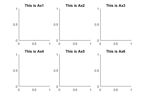
Matlab has a function for creating figures with multiple subplots. Logically, this function is called ‘subplot’ – check the subplot documentation for information. Basically, the subplot function needs three inputs: number of elements vertically, number of element horizontally and the element index you want to create an plot in. The concept is illustrated in the following example:
Fig=figure('Position',[200 200 600 400]); % Definde the figure (Fig will be its handle)
% 2 x 3 subplots are created.
Ax1=subplot(2,3,1); title('This is Ax1'); % Subplot element 1 will be occupied by Ax1
Ax2=subplot(2,3,2); title('This is Ax2'); % Subplot element 2 will be occupied by Ax2
Ax3=subplot(2,3,3); title('This is Ax3'); % Subplot element 3 will be occupied by Ax3
Ax4=subplot(2,3,4); title('This is Ax4'); % Subplot element 4 will be occupied by Ax4
Ax5=subplot(2,3,5); title('This is Ax5'); % Subplot element 5 will be occupied by Ax5
Ax6=subplot(2,3,6); title('This is Ax6'); % Subplot element 6 will be occupied by Ax6
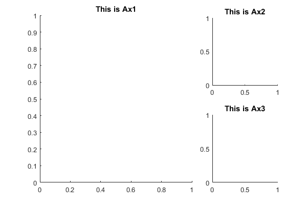
If you want to create subplots with different sizes in the figure, you can also choose to address the axes to several of the subplot elements:
Fig=figure('Position',[200 200 600 400]); % Definde the figure (Fig will be its handle)
% 2 x 3 subplots are created, but the elements will be occupied by only three axes.
Ax1=subplot(2,3,[1 2 4 5]); title('This is Ax1'); % Subplot element 1,2,4,5 will be occupied by Ax1
Ax2=subplot(2,3,3); title('This is Ax2'); % Subplot element 3 will be occupied by Ax2
Ax3=subplot(2,3,6); title('This is Ax3'); % Subplot element 6 will be occupied by Ax3
Task
Use the 'subplot' function to create an animation visualizing the shallow wave model in more than one plot. Save it as an avi or gif movie. You decide what and how much you want to show - as long the animation consists of at least two plots.
For inspiration an example containing four plots; 3d surface plot, 2d filled contour plot, line graphic showing the maximum and minimum water depth, and a bar plot the water depth distribution.
Part 2 - 3D Animation with changing view point and zoom level
Changing the view and zoom of your plot during the animation makes is possible to visualize different part of your model result at different times. A side effect is that the changing view makes your animation more dynamic and cool :). However, changing the view and zoom in a coordinated way during the animation is far from trivial and require creativity.
Background
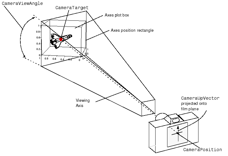
If you want to have the total control over how your 3D graphic is displayed, you need to specify quite a few properties for your plot axes. When 3D graphic is displayed in your Matlab figure, it is viewed from a specific direction from a point in space.
(Matlab, 2012)
You will view your plot form the 'CameraPosition' point and the 'CameraTarget' specifies the direction of the view. The 'CameraViewAngle' will determine how large the plot appears in the figure. Changing 'CameraPosition' and maybe also the 'CameraTarget' during the animation, will have the same effect as moving a camera around the 3D-plot. Consequently, changing the 'CameraViewAnige' will have the same effect as zooming on the camera.
The ‘CameraPosition’,‘CameraTarget’ and ‘CameraViewAngle’ is found within axes properties and can easily be changed using the 'set' function (if you know the handle to axes). The following example illustrates how you finds the the current values and how you can change them using the 'get' and 'set' functions:
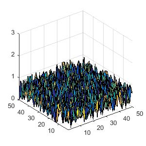
H=rand(50); % Get some data to plot in 3D (50 x 50 matrix of random numbers between 0 and 1)
Fig=figure('position',[200 200 300 300]); % Create figure with the handle 'Fig'
Ax=axes; % Create axes with the handle 'Ax'
Plot3D=surf(H); % Plot the surface
axis(Ax,[1 50 1 50 0 3]); % Set axis limit
CamPos=get(Ax,'CameraPosition') % Get CameraPosition
CamTarget=get(Ax,'CameraTarget') % CameraTarget
ViewAngle=get(Ax,'CameraViewAngle') % CameraViewAngle
CamPos =

 -198.2198 -266.0574   14.4904


CamTarget =

   25.5000   25.5000    1.5000


ViewAngle =

   10.3396
It is now easy to make changes using the 'set' function:
set(Ax,'CameraPosition',[200 -327 4.6]); % Set CameraPosition
set(Ax,'CameraViewAngle',5); % Set CameraViewAngle
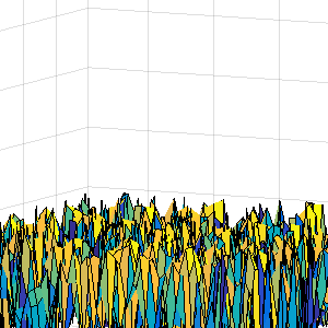
As you can see - it is in principle very simple to change view and zoom of a 3D plot. The difficult part is to find out, what the changes should be and make the changes coordinated and smoothly in the animation. As the 'CameraPosition' and 'CameraTarget' is points in the space with coordinats according to the plot axes, is can be tricky to imagine the consequences of a change.
Conveniently, Matlab have some helping functions called 'view' and 'camzoom'. These functions automate the process and make the changes more transparent and imaginable. But with automation comes a minor lack of control; so if you want handle all the aspects of the view completely, use the method described above. Otherwise, use the 'view' and 'camzoom' functions. For most purposes they are sufficient anyway.
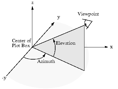
The 'view' function defines the viewpoint polarly by an azimuth angle and an elevation angle. Thereby, rotating the plot during the animation becomes quite simple - For example just vary the azimuth linearly during animation will create and rotating anmation.
(Matlab, 2012)
The 'camzoom' zooms in and out - if the zoom factor is smaller than one you will zoom out and if is greater than one you will zoom in. Type ‘doc camzoom‘ in your command window to view the documentation.
Although, the 'view' and 'camzoom' functions makes it much easier to understand and make the changed to the view of the 3d plot, you will still need to figure out how to coordinate your changed in a smooth way for your animation. This final step requires some creativity and maybe also some experience. The following example illustrate how time series for the view (azimuth and elevation angle time series) and zoom (zoomfactor) can be achieved. It is only an example and there is no "right" or "wrong" way of doing it.
H=rand(50); % Get some data to plot in 3D (50 x 50 matrix of random numbers between 0 and 1)
Fig2=figure('position',[200 200 400 400]); % Create figure with the handle Fig2
Ax2=axes; % Create axes with the handle Ax
Plot3D=surf(H); % Plot the surface
axis(Ax2,[1 50 1 50 0 3]); % Set axis limit

SimTime=25;
dt=0.1;

% Definding the timeserie for the camera wiev point
azTS=linspace(1,180,round(SimTime/dt));
% During the 30 sec simulation the viwepoint azimuth will change linearly
% from 1 deg to 180 deg
elTS=sind(azTS-5)*60;
% During the 30 sec simulation the view point elevation angle change as a
% sinus curve form -4 deg peak at 60 deg and end at 5 deg

% Definding the timeserie for camera zoom
zoomTS=(sind(azTS)*0.01)+(1-0.013/2);
% During the 30 sec simulation the camera zoom changes as a sinus curve
% form 0.9937 peak at 1.0035 deg and end 0.9937 (Values smaler than one
% zooms out values larger the one zooms in)

for i=1:SimTime/dt
    view(Ax2,[azTS(i),elTS(i)]); % Change the view point
    camzoom(Ax2,zoomTS(i)); % Change the zoom
    pause(0.01); % Delay to show the figure
end
close(Fig2);
If you copy the piece of code in to your command window this animation with changing view and zoom should appear:

Refresh your browser to restart the animation.
Task
Use the view and maybe also the zoom command to make an animation of the shallow water wave model, where the view and perhaps also zoom are changed during the animation. As a starting point you can try to see if you can fit in the azimuth, elevation and zoomfactor time series from the example above.
This will give you an animation similar to this.