Exercise 1 - Animation of Radar Data
By Jesper Ellerbæk Nielsen
During this exercise you will make an animation of rainfall passing Denmark. The rainfall is measured by the c-band radar located in Virring.
The execise focuses on how data can be presented as an overlay and which options you have, when you want to make an animation.
Contents
Introduction
For the purpose of this exercise one week of radar data is available for download here. Note that the data is zip-compressed and need to be uncompressed before use. Beneficially, you can unzip the radar data into the same folder you are working in. This will make it easier to access the data.
The archive of the radar data is structured in a folder structure. Data with timestamp 15:00 from the 18th of July 2012 is located in: /Virring/2012/07/18. The name of the file is ekxv1500.wrk, where ‘ekxv’ is the identifying prefix for the Virring c-band radar. The ‘.wkr’ file format is the binary file format DMI uses for their data products. In order to load a radar data set into Matlab you will need a reader-function, which is available for download here. Extract the ‘LoadWRKFile.m’ from the zip-file into the folder you are working in and you will be able to call the reader-function from your exercise code.
The function call for loading the radar data into Matlab is strait forward. You just need to specify the file-path of the .wrk file and you will get the radar data into your workspace. Function syntax: Data=LoadWRKfile(FilePath)
Try to load the data set from 18th of July 2012 15:00 and use the imagesc plot function to view the radar data:
FilePath='Virring\2012\07\18\ekxv1500.wrk'; % Definding the file path.
Data=LoadWRKFile(FilePath); % Load the radar data using the LoadWRKFile function.
imagesc(Data); % Plot an image of the data.
axis image; % Secures that the proportion in the x and y direction is equal.
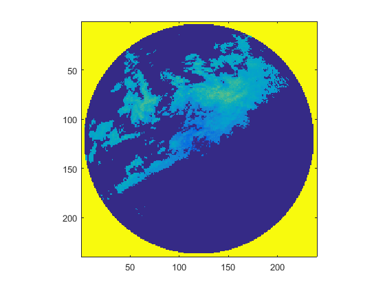
You can always get more information on the Matlab function from the documentation. The documentation can easy be accessed by typing help followed by the function name. Try this now with the imagesc function:
help imagesc;
 IMAGESC Scale data and display as image.
    IMAGESC(...) is the same as IMAGE(...) except the data is scaled
    to use the full colormap.

    IMAGESC(...,CLIM) where CLIM = [CLOW CHIGH] can specify the
    scaling.

    See also IMSHOW,IMAGE, COLORBAR, IMREAD, IMWRITE.

    Reference page for imagesc
Matlab automatically suggests other related function, which might be of relevance for you. You can access their documentation simply by clicking the links. When you use the help command as shown above, you will only get the most essential part of the documentation printed out in the command window. If you want to read the full documentation for a function, just click the 'doc' link (in this case doc imagesc) and the full Matlab documentation will pop-up in a separate window. Here, you will find additional information and often helpful code-examples. This is equivalent to typing 'doc imagesc' directly in the the command window.
Google is also convenient for getting information and examples of Matlab functions. Especially, if you need a function you don’t know the name of or if you have troubles finding what you are searching for in the documentation. Just add 'matlab' in the Google search request and you will almost always get something relevant – there is always someone who has faced the same matlab coding problem as you.
Now you are almost ready for making radar animations – you are able to load the radar data and you know how to get help and find the documentation. But before you are compleatly set for working with radar data, you will need to transform the echoes in the data to rain intensities.
Reviewing the detailed aspects of weather radar measurements are beyond the scope of this exercise. However, you will (if not already) be introduced to this type of precipitation measurement in the course 'Urban Hydroinformatics'. Anyway, what you need to know for now is that the .wrk file contain a 8-bit rescaled version of the measured radar reflectivity in the atmosphere. This means, that the data you have already loaded and plotted, only contains values (counts) between 0 and 255. 255 is a dummy-value indicating that there is no measurement in the pixel (no-data). These dummy-values are the reason you get the yellow area around the data as shown above. All cells beyond 240 km from the radar are assigned the no-data value, because it is the maximum range of the radar. Consequently, the radar is located in the center of the data matrix. If you take look on the size of the data matrix you will find that is a 240x240 matrix.
size(Data); % This function returns the size of the matrix. You can also find this information in the workspace.
Each cell (element) of the matrix represents an area of 2 x 2 km which consequently, gives the maximum range of 240km in the horizontal and vertical direction of the matrix.
The counts of the radar data are transformed linearly to the real radar reflectivity of the atmosphere in dBz by an offset and slope factor:


The outcome of this is the measured radar reflectivity of the atmosphere in the logarithmic decibel scale. This measure need to be transformed to reflectivity in a linear z scale:

The final transformation of the linear reflectivity z into rain intensity is done by an empirical power law function with standard Marshall-Palmer parameters (Marshall and Palmer, 1948):

Where z is the linear reflectivity, R is the rainfall intensity in mm/hr, and A and b is the empirical power law parameters, with the standard Marshall-Palmer values of:


Due to the logarithmic nature of the radar data, every cell will end up containing at least a tiny fraction of precipitation. The linear reflectivity cannot be zero but only very small when it is transformed from the logarithmic decibel scale. Therefore, a threshold is often applied to filter transformations artifacts from the precipitation. A threshold of 1 mm^6 is appropriate in most cases.
Try to apply these transformations and relation to your loaded radar data and plot the data again:
Data(find(Data==255))=0; %This gets rid of the dummy values. Type help find for more info.

alpha=0.5; % set slope factor
beta=-32; % set offset factor
Data=(Data.*alpha)+beta; % Transform count to dBz. The '.' in front of '*' treats
% every elements of the matrix separately and thereby ignore the build in
% matrix algebra Matlab normally uses. (In this case, this makes no
% difference as alpha is a factor. Type 'help .*' for more information)

Data=10.^(Data./10); % Transform dBz to linear z.
Data(find(Data<1))=0; % Threshold for precipitation.
PalmerA=200; % set the A parameter
Palmerb=1.6; % set the b parameter
Data=(Data./PalmerA).^(1/Palmerb); % Transform the linear z to rain intensity

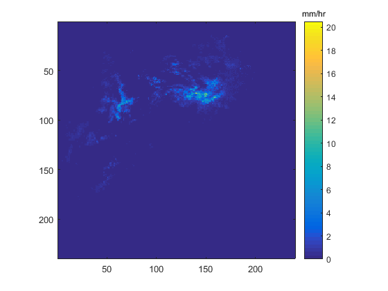
imagesc(Data); % plot the rainintensity
axis image;
bar=colorbar; % add a color bar and store its handle in order to add a title to it
title(bar,'mm/hr'); % add the unit to the colorbar
Part 1 - Make an animation of the radar data
In order to get started with you animation you need to make a routine which loads and transform the radar data one file after the other. For this purpose a 'for loop' might be convenient. If you are not familiar with 'for loops' in Matlab type 'help for' to get some information.
The provided set of radar data runs from 18th of July 00:00 to the 24th of July 2012 23:50. The temporal resolution of the data is 10 minutes.
The functions 'datestr' and 'datenum' are useful in constructing the numerous filepaths needed to load the radar data. 'datenum' converts a date string to the number days from a reference data. 'datestr' converts the date number back to a date string. See the documentation for information.
Hint: example on how 'datestr' and 'datenum' can be used:
time=datenum('2012-07-18 1450','yyyy-mm-dd HHMM'); % Converting a date string to a date number
path=datestr(time,'Virring\\yyyy\\mm\\dd\\ekxvHHMM.wrk');% Constructing a filepath by the help of the datastr function
disp(path); % Display the filepath see below
time=time+1/(24*60)*10; % Add 10 minuts to the date number
path=datestr(time,'Virring\\yyyy\\mm\\dd\\ekxvHHMM.wrk');% Constructing the next filepath
disp(path); % Display the filepath see below
Virring\2012\07\18\ekxv1450.wrk
Virring\2012\07\18\ekxv1500.wrk
Furthermore, you might need to evaluate whether or not the radar data you are trying to load actually exists. It is quite common that a set of data is missing and the load function will then fail. For this purpose the 'exist' function might be useful combined with an 'if statement'. Type 'help if' and 'help exist' for more info if needed.
Task
Make a for loop which loads one radar data-set after the other and converts the data to rain intensities. Then add a pause and the 'imagesc' function to the loop and you will get your first animation of radar data in Matlab :). The pause is needed in order to view the plot on your screen. Otherwise, the animation will be so fast, that you will not be able to see it. Type 'help pause' to figure out how the 'pause' function works.
Your result should look like this:
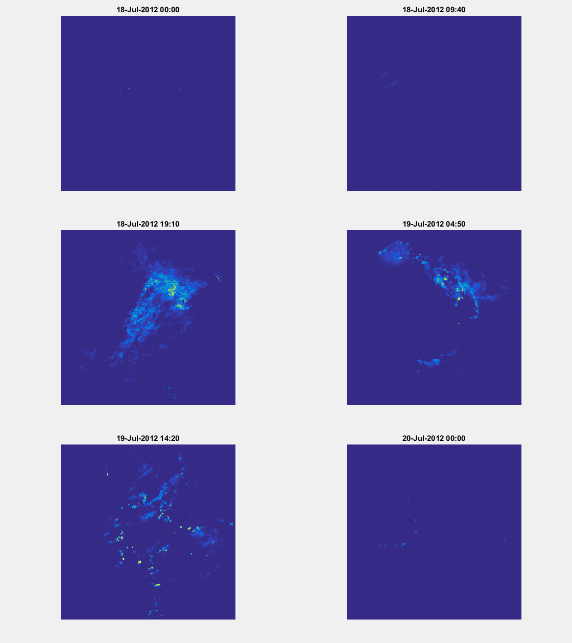
You can add the timestamp as the plot title by using the title command and remove the axis as they are not very meaningful anyway. Furthermore, you might want to set fixed limits on the color-range. Otherwise, every image in your animation will have a individual scale from the minmum to the maximum value of the data set.
imagesc(Data,[0 10]); % Plot the rainintensity with limits
axis image;
axis off; % Hide the axis
title(datestr(time,'dd-mmm-yyyy MM:HH')); % Add timestamp as title
pause(0.05); % Wait for a while in order to display the figure
close(gcf);
Part 2 - Make the animation more informative and save it as a gif animation
In this second part of the exercise, you will make the animation more informative by adding a background map for geographical reference and save the animation as a GIF-animation (Graphics Interchange Format). The GIF-format benefits of being almost universal – if you make a GIF-animation you are almost certain that everybody will be able to view your animation. For presentations in PowerPoint inserted GIF animations will automatically be imbedded in the presentation file. Thereby, you don’t need to worry about copying the animation file or where your animations are located on the computer, if you need to transfer your PowerPoint presentation to another computer. This will save you from akward moments, when you present your fantastic work :).
GIF has on the other side also limitations. It is based on an 8-bit-per-pixel bitmap-image format, therefore only 256 different colors can be displayed in the animations. For many applications (like the one in this exercise) 8-bit is sufficient. However, if you are working with lifelike colors and colored shadings e.g. images from a digital camera, 8-bit colors may be insufficient. Another downside with GIF-animations are that you cannot pause, rewind etc. the animations. Furthermore, long animations with large images tends to be quite slow.
Matlab facilitates many of the common animation and movie formats. In this part of the exercise you will get experience with GIF while the following will introduce you to avi. You will of course always have the option of using third-party software to combine images produced by Matlab into an animation e.g. Windows MovieMaker.
NOTE: if you experience problems with tranparancy or mirrored text on axes and titles - do not panic. This is a known problem of some ATI graphic devices combined with Matlab. You can solve this problem by typing this command in the command window:
opengl('software')
However, wait until you experience problems. If not, there is no need to enter the command.
Creating the animation for this part of the exercise is basically a two step procedure. First you make the animation of the radar data as the overlay, and then you add the required code for saving the animation as GIF.
Create a plot of the radar data as an overlay on a map
For of this part of the exercise download this background map of Denmark and save it into the folder you are working in. The map fits the covered area of the Virring c-band radar, which is located in the center of the map.
In this part of the exercise, it is important that you keep track of all handles in the figure (figure handle, axes handle, plot handle etc.). One way of making an overlayed plot in Matlab is by making two plot axes on top of each other. As Matlab automatically tries to add your commands to the 'current' figure or axis, it is important the you are able to explain Matlab what you want to change or add with your commands. I order to do so, you need to handle the handles with care.
The benefit of this effort is that you will be able to make much more complex plots. You will also be able to make animations much faster, as you will only change what needs to be changed between frames instead of building the whole figure from scratch.
For the overlay plot you will basically be using two Matlab functions: 'imread' to load the background map, and 'imagesc' plot function for plotting both the map and the radar data. However, you also need to set the transparency of the radar data in order to see the underlaying map. You can get information about transparency by typing 'help alpha' in the command window. See also the documentation for 'imread' and 'imagesc' if needed.
The map can simply be loaded and plotted by
Fig=figure;
BackgroundMAP=imread('Virring240km.jpg');
Map=imagesc(BackgroundMAP);
axis image;
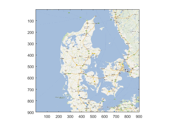
If you carefully construct your plot and keep track of the handles, it is easy the to change the figure afterwards. The following example illustrates this concept and plots the radar image on top of the map.
Fig=figure('position',[50 50 700 700]); % Creates the figure
BackgrounfAx=axes; % Set axes for background picture
Map=imagesc(BackgroundMAP); % Plots the background map
set(BackgrounfAx,'handlevisibility','off','visible','off','DataAspectRatio',[1,1,1]);
%This sets the axes property, so that the axes is invisible and the
%DataAspectRatio = [1,1,1] is the same as axis image.
RadarAx=axes; % Set the axis on top of the background map
alpha_data=(Data>0).*0.5;% define the transparency (cells with no rain will
% be completly transparant and cells with pricipitation will be 50%
% transparent.
RainData=imagesc(Data,'Parent',RadarAx,'AlphaData',alpha_data,[0 15]); % Plots the
% radar data with transparency according to alpha_data
set(RadarAx,'handlevisibility','off','visible','off','DataAspectRatio',[1,1,1]); % Removes the axis and
%image the axis
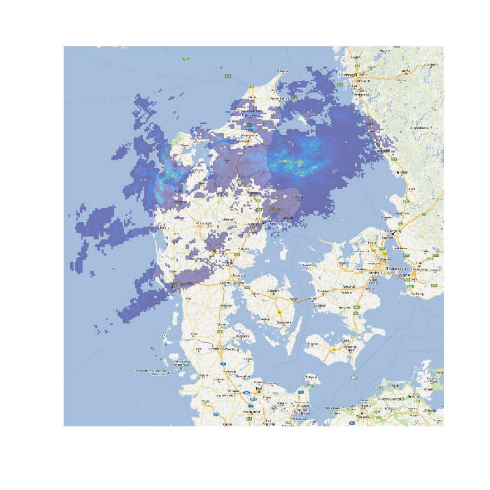
You can now easy change the content of the plot by using the 'set' function:
set(Fig,'position',[50 50 300 300]) % This makes the figure smaller
set(Map,'Cdata',imrotate(BackgroundMAP,90))% This will repalce the map with a rotated version
set(RainData,'Cdata',Data*10)% This will replace the radar data
drawnow % This command is not always be needed
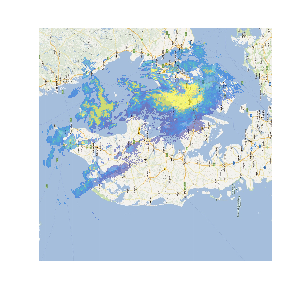
Hint: If you want to know what can be adjusted for a specific object, the 'get' function is very helpful. This function returns the current settings and properties of the object:
Temp=get(Fig); %Properties of 'Fig' are saved in 'Temp'
In this case, 'Temp' will contain all the properties and settings of the 'Fig' object.
You are now ready for creating the animation! Combining the above example (or similar) with the 'for loop' from part 1. Make a animation of the radar data with an underlaying map.
The result should look something like this:
Save your animation as GIF
The final step in this exercise is to save your newly created animation as a GIF.
Making a GIF animation in Matlab may appear complicated at first, however, when you get to know the required functions and how they are used in combination, it is fairly strait forward. Although, there are several slightly different ways of making the animation, the following example will be based on four Matlab functions.
- getframe
- frame2im
- rgb2ind
- imwrite
The 'getframe' function grabs the figure or axes and returns a movie frame. This function is universal and is used for several types of animations. In contrast, the remaining three functions is specific for GIF animations. See the documentation for details on the four functions.
The 'frame2im' and 'rgb2ind' are used to convert the movie frames into images with the right properties. Otherwise, they cannot be written to the GIF file by the imwrite function. 'frame2im' is used to retrieve an indexed image from the movie frame. The result is the same type of 3d matrix you got, when you loaded the background map with 'imread'.
The frame and thereby the image retrieved (by mean of frame2im) is a true-color image. True-color images have the possibility to contain 16.7 million different colors, therefore, the colors of the image needs to be compressed to 8-bit (256 colors) to fit the GIF format. This can be achieved by the 'rgb2ind' function.
This process will of cause reduce the number of possible colors in the image however, the effect on the image quality is limited as exemplified:
figure('position',[50 50 1050 330]);
ImgTrue=imread('marie.jpg');
[Img8bit,cm8bit] = rgb2ind(ImgTrue,256);
AxisTrue=subplot(1,2,1);
Axes8bit=subplot(1,2,2);
PlotTrue=imagesc(ImgTrue,'Parent',AxisTrue);
Plot8bit=imagesc(Img8bit,'Parent',Axes8bit);
colormap(Axes8bit,cm8bit);
title(AxisTrue,'True Colors');
title(Axes8bit,'256 Colors');
axis([AxisTrue Axes8bit],'image','off');

The 'imwrite' function is a bit trickier to use. First the GIF-file need to be created with the first image and then the rest of the images are appended to the file. The following example illustrates this concept and is manly inspired by the example in the Matlab documentation.
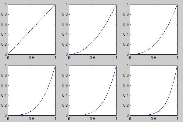
x = 0:0.01:1;
H=figure('position',[200 200 200 200]);
filename = 'example.gif';
for n = 1:0.5:5
y = x.^n;
plot(x,y);
drawnow;
frame = getframe(H); % Grab the frame with getframe
im = frame2im(frame); % The frame is converted to an indexed image
[imind,cm] = rgb2ind(im,256); % The image is compressed to 8-bit
pause(0.05);
%Dependent on how fast your computer is, you might need to include a pause
%in your script. This will insure that your computer will have enough time
%to write the file properly.
if n == 1;
imwrite(imind,cm,filename,'gif', 'Loopcount',inf); % The first image is used to create the GIF file
else
imwrite(imind,cm,filename,'gif','WriteMode','append'); % The rest of the images is appended
end
end
close(H); % Close the figure when done
Try to run this example and you should get this GIF animation:
Task
Use the concept from the example above in your animation code and save the radar data animation with background map as a GIF. You might want to change the display time of the animation in order to make it faster. Consult the Matlab documentation or Google for the necessary information. Feel free to put your personal touch on the animation to make it cooler.