MATLAB Lecture 01 - Exercises - 2D graph visualization

By Malte Ahm / Jesper Ellerbæk Nielsen - jen@civil.aau.dk

In these exercises you will deal with different types of data which you have to load and plot in different ways.

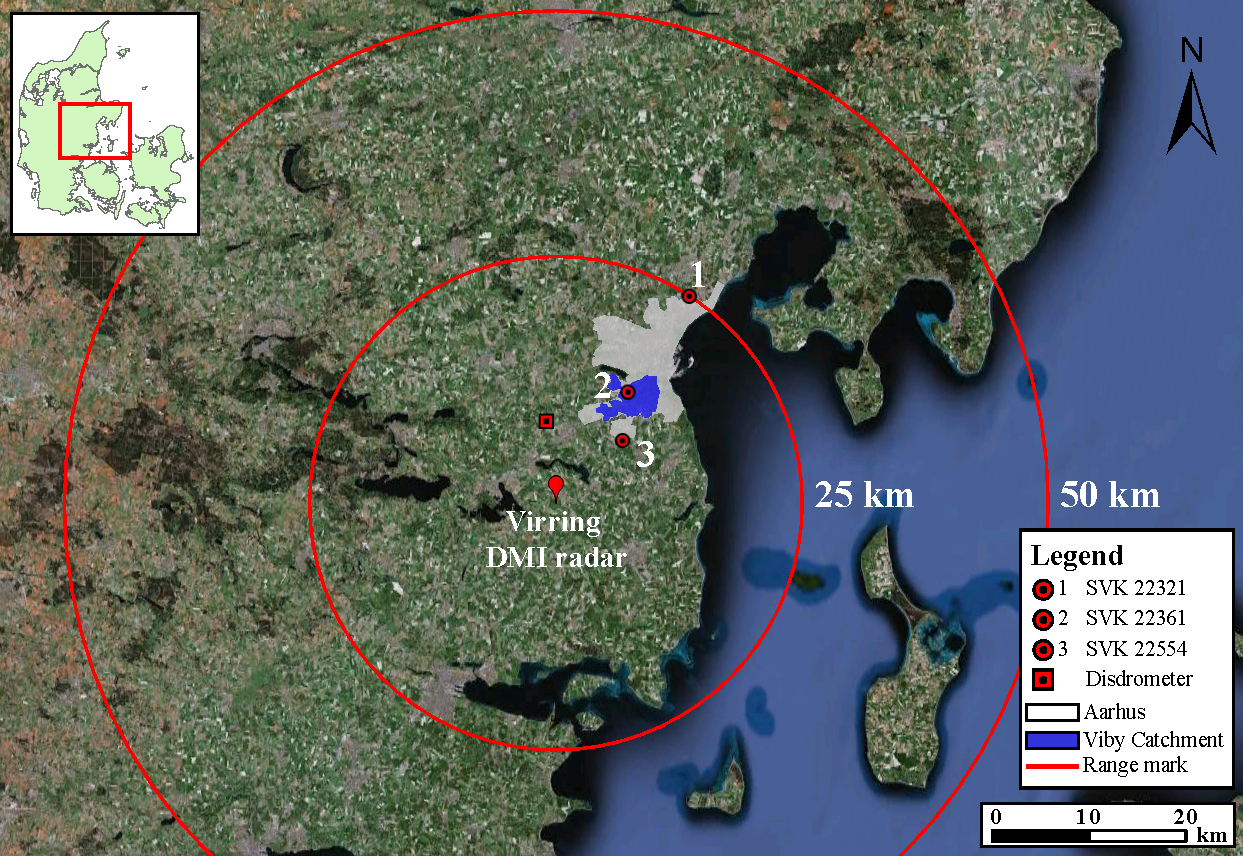
The case area which you are going to work with today is shown in the figure below. The case area is called the Viby Catchment and is located in municipality of Aarhus.

The requirements for the hand-in of the solution are as following:

A video demostration of the build-in publishing tool in MATLAB can be found be found here:

Video demostration of the publishing tool

The three exercises for MATLAB Lecture 01 is setup so you with advantage can answer all exercises by using the same MATLAB file and thereby save many lines of code and time.

Tip: When plotting rain gauge and radar data it can be an idea to use the plot function "stairs" instead of the function "plot".

Contents

Exercise 01 - Load and plot rain gauge data

In this exercise you will deal with the topic of loading and plotting rain gauge data from the danish national rain gauge network SVK. Rain gauge data from this network is often acquired in the KM2 file format (*.km2). We will therefore first have to load the data from this data format.

The data used for this exercise can be downloaded here:

Download rain gauge data here!

The function used for loading the rain gauge data from the KM2 file format and transforming them into a continues time series can be downloaded here:

Download LoadSVK_TS.m function here!

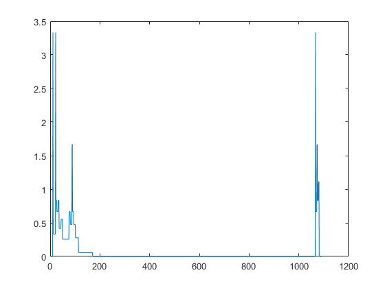
Spend some time reviewing the code to get a feeling of what is going on and what the output is. Try to load the data from the rain gauge SVK22321 and plot the data using the function "plot".

% Rain gauge files
SVK22321_path='SVK22321_20120718_20120725.km2';
% Load rain data
SVK22321_data=LoadSVK_TS(SVK22321_path);
% Plot data
plot(SVK22321_data(:,2))

Now the aim of this exercise is to plot all three time series for the three rain gauge in the same plot with different colors and line style, legend, title, axes title, and date formatted tick labels on the x-axis.

A figure like this should be obtained. Remeber to limit the axes.

As you maybe already have lurked the unit of the rain gauge data in the KM2 files is . We want the unit to be , so remember to recalculate the data before plotting it.

Remember to use handles when plotting. Experiences of using handels will benefit you later. Use the function "figure" to create a figure handle, the function "axes" to create an axes handle, and the selected plot function to create a 2D graph handle.

Exercise 02a - Load and plot weather radar data

In this exercise you will deal with the topic of loading and plotting time series of specific weather radar data pixels from the C-band radar located in Virring south-west of Aahurs.

The data needed for this exercise can be downloaded here:

Download weather radar data here!

The weather radar data are stored in a compressed file and you will therefore need to uncompress the data before you can use them. If you store the uncompressed data in you working directory it will be easier for you to access them.

The archive structure of the weather radar data consist of some different subfolders. An example of thisw structure is given here: Data with timestamp 15:00 from the 18th of July 2012 is located in: /Virring/2012/07/18. The name of the file is ekxv1500.wrk, where ‘ekxv’ is the identifying prefix for the Virring C-band radar.

The file format for the weather radar data is a binary format "*.wrk" used by DMI (Danish Meteorological Institute) for their CAPPI data products. A function is here provided to read the binary weather radar format:

Download LoadRadarWRKFile.m function here!

You will need to call this function in a for-loop to load the data into your program. The easiest way to load these data is first to create a column vector with all the time stamps you need to load and an empty 3D matrix to store the loaded data.

Spend some time reviewing the function code to get a feeling of what is going on and what the output is.

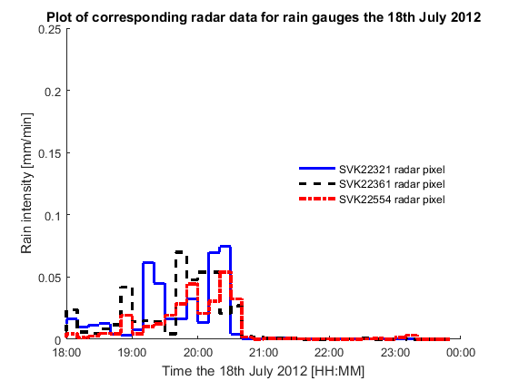
Now the aim of this exercise is to plot the three time series for the radar pixels corresponding to the location of the three rain gauges. The cell positions in the data is given here:

A figure like this should be obtained. Remeber to limit the axes.

Exercise 02b - Plot rain gauge and weather radar data

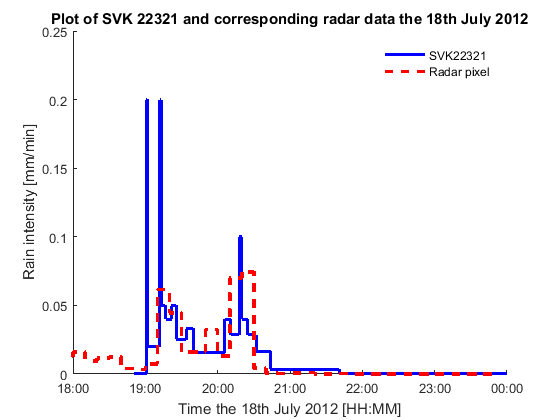
In this exercise you will deal with the topic of plotting rain gauge and weather radar data together. Plot the rain gauge data for SVK22361 along with the time series for the corresponding weather radar pixel.

A figure like this should be obtained. Remeber to limit the axes.

Exercise 03 - Load flow data and plot these along with rain gauge and weather radar data

In this exercise you will deal with the topic of loading and plotting flow measurement time series along with rain gauge data and weather radar from the corresponding data pixels.

The data needed for this exercise can be downloaded here:

Download flow measurement data from Viby WWTP here!

The flow data are stored in a Microsoft Office Excel file (*.xlsx) and you will have to load it from this file. To be able to plot the data correct you will both need to load the time stamps and the inlet flow data. Since the time stamps are text strings and the data are doubles you will need to load each column seperatly. Afterwards you will need to transforme the time stamps text strings to datenum time stamps to be able to use them for the plot functions.

You can use this peice of code to transform the time stamps to datenum:

   % Transforme time stamp strings to datenum time stamps (proces is slow)
   FlowTimeStamps=zeros(size(FlowTimeStampStrings,1),1);
   for n=1:size(FlowTimeStampStrings,1)
       try
           FlowTimeStamps(n)=datenum(FlowTimeStampStrings(n), 'dd-mm-yyyy HH:MM:SS');
       catch err
           FlowTimeStamps(n)=datenum(FlowTimeStampStrings(n), 'dd-mm-yyyy');
       end
   end

Spend some time reviewing this piece of code to get a feeling of what is going on and way we have transforme the time stamps in this way.

A figure like this should be obtained. Remeber to limit the axes.

Documentation for the main functions used for the solution - REALLY GOOD IDEA TO LOOK AT THIS IF YOU ARE LOST!

A good way to find help for MATLAB function is by the use of www.google.com. E.g. by writing "MATLAB figure" in the search field.

Another way, if you know the function, is to write "help" followed by the function name in the command windows in MATLAB. E.g. "help function".

Exercise 1

figure

hold

stairs

axes (used in combination with "get")

get

set

linespec (Line Specification)

colorspec (Color Specification)

axis

datetick

xlabel

ylabel

legend

title

Exercise 2 - only new functions

datenum

if/elseif/else

while

for

zeros

Exercise 3 - only new functions

xlsread

Well, to challenge you a bit and force you to use www.google.com I will not reveal which functions I have used for plotting the data with multiple axes. However I can reveal for you, that it is very important to control your plotting handles in this exercise.

Information about axes properties

Other usefull function to minimize the computational time of you script

save

load

Exercises created for the course visualization by Malte Ahm - ma@civil.aau.dk

Published with MATLAB® R2015b