Exercise 1 - Recognition of Handwritten Digits

By Jesper Ellerbæk Nielsen

In this exercise, you will create and train a neural network that can recognise the patterns of handwritten digits.

The exercise focus on the fundamental aspects of creating, training and using Neural Networks in Matlab.

Contents

Introduction

Working with Neural Networks for machine learning require data – lots of data! Luckily for us, there exist a large database, containing handwritten digits. The database is called the MNIST database and can be found several places on the internet. You can read more about the database on this website yann.lecun.com/exdb/mnist/ The database consists of two datasets. A training dataset containing 60,000 digits and a test dataset with 10.000 digits. Both datasets come of course with labels specifying the correct answer.

The digits have been size-normalized and centred in a fixed-size image of 28x28 pixels, and the database was created for people who want to try learning techniques and pattern recognition methods on real-world data while spending minimal efforts on preprocessing and formatting.

You can find the database on the course Moodle page, which you need to copy to your working directory in Matlab for this exercise. The files you will be looking for are named:

The two first contains the training 60,000 images and labels, and the two last files are containing 10,000 test images and labels, that can be used to test the performance of the Neural Network when it is trained.

The files are written in a specific binary format as described on the MNIST website yann.lecun.com/exdb/mnist/. But to ease the process of loading the files into Matlab, I have written a load function, that can do this trivial work for you. Like the database the loading function is also avaliable for download no the course Moodle page, named:

Download the function and save it in your working directory in Matlab.

Part 1 - Loading the MNIST training data

The loading function loads both the images and associated labels at once. However, you need to specify first the file with images followed by the label file. It takes a few seconds to load the data, however when done, you will be notified in the Command Window.

% Loading training images and labels
imageFile='train-images.idx3-ubyte';
labelFile='train-labels.idx1-ubyte';
[images,labels] = loadMNISTdata(imageFile,labelFile);

Loading digit images..
File contains 60000 digit images
Done

Loading labels..
File contains 60000 images labels
Done

The output from the loading function [images,labels] is the images and labels as the names suggest. The digits images are loaded into a 3D matrix with the dimension of 28 x 28 x 60.000, where each element in the third dimension is an image, as illustrated hereunder:

% The dimension (size) of the loaded training images
disp(size(images));

          28          28       60000

The labels are loaded into a column vector with 60.000 elements, in the same order as the digits images.

% The dimension (size) of loaded training labels
disp(size(labels));

       60000           1

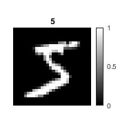
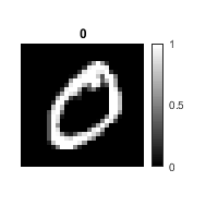
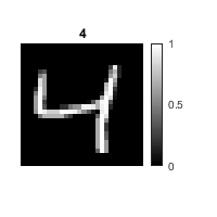
You can show a digit image by using the imagesc or the imshow function. Here is exemplified who you can visualise the three first image of the database and use its labelled value in the title:

% Displaying the three first images
for i=1:3
    figure('position',[500 500 200 200]);
    Img=images(:,:,i);
    Lbl=labels(i);
    imagesc(Img);
    colormap('gray');
    colorbar;
    axis image off
    title(num2str(Lbl));
end

Spend some time to examining the data you have loaded, so you get an understanding of how they are structured.

Part 2 - Structuring the training data correctly

The Neural Network cannot use the 3D matrix structure of the digit images, so you need to transform all the images into a 2D-matrix (784x60000), where each column contain pixel values form each of the training images. This is simply done by stacking all the 28 columns of the training image so that each image becomes a 28x28=784 column vector. In Matlab, this operation can be done in several ways, but one way is to use the inbuild function reshape.

To help you get started, I have hereunder exemplified how the first image can be transformed into a column vector by the reshape function. You need to figure out a way to do it for the rest of the images so that all the images are turned into columns next to each other.

% Reshapeing the 28x28 image in to a column vector
Col_img=reshape(images(:,:,1),[],1);

Like the training image data, the training label data is not structured correctly for the Neural Network application. When loaded, the label data is simply the number, the handwritten digit represents. However, you need to structure the labels in a classification way of thinking, meaning that each label is turned in to a 10 element column vector, where the 1st element is 1, and the rest is 0, if the labelled value is zero. The 2nd element is 1 and the rest is zero, if the labelled is 1 and so on, e.g.:

  [2]   [3]   [0]   [9]
   0     0     1     0
   0     0     0     0
   1     0     0     0
   0     1     0     0
   0     0     0     0
   0     0     0     0
   0     0     0     0
   0     0     0     0
   0     0     0     0
   0     0     0     1

You need figure out how to transform the label data into a 2D-matrix (10x60000), where each column represents a label by at categorising vector.

Part 3 - Creating the Neural network

Your training data is now ready to use in Neural Network machine learning. For this, you need at Neural Network to train. In Matlab, an empty custom Neural Network is created by the function network. The many inputs control how the network is structured with layers and connections and might be a bit counterintuitive, in the beginning.

   net = network(numInputs, numLayers, biasConnect, inputConnect, layerConnect, outputConnect)

Remember you can always get the documentation for a function by typing doc followed by the function name in the Command window:

% Open the documentations of the network function
doc network

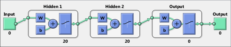
Here is shown how to generate a standard Neural Network with input three hidden layers and an output layer, with no added thrills. Moreover, it is shown how you can use the view to visualise the Neural Network.

% Create a custom neural network with four layers
net1=network(1,4,[1; 1; 1; 1],[1; 0; 0; 0],[0 0 0 0;1 0 0 0;0 1 0 0; 0 0 1 0],[0 0 0 1]);
% Rename the layers
net1.layers{1}.name='Hidden Layer 1';
net1.layers{2}.name='Hidden Layer 2';
net1.layers{3}.name='Hidden Layer 3';
net1.layers{4}.name='Output Layer';
% View the network
view(net1);

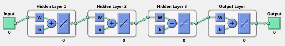
As you can see, by default, the network function generates an almost empty network. For example, there are 0 neurons in the three hidden layers, and all the network layers use linear neuron function to translate the input from the previous layer to the next. Therefore, quite a lot need to be specified and adjusted before the network can be trained.

But before you go to the next part, figure out how you can use the network function to generate a network similar to the above, but with only two hidden layers.

Part 4 - Configuring the Neural Network

The network function store the Neural Network in a 'network container' as its output. This 'network container' control and contains all information and aspects about the Neural Network, for example how the layers are connected, the number of neurons in each layer, which neuron function is used in which layers, which minimisation algorithm and cost function used in training etc. The easiest way to access its content is simply by typing the network name in the command window, and its contest will be shown. In the command window, you will get links to the documentation for every element of the network.

Try to type your network name into the command window and press enter. Then click on 'layers' to see what the layers consist of. Then click the 'transferFcn' to get information about the neuron functions. Lastly, click on the 'transfer function' link to see which transfer function is available as neuron functions in Matlab.

The way the network elements is configured is by addressing the network as a structure. For example, the number of neurons in the two hidden layers can be set like this:

% Set the number of neuron in hidden layer 1 to 20
net.layers{1}.size=20;
% Set the number of neuron in hidden layer 2 to 20
net.layers{2}.size=20;

You can always get or see the current value or setting simply by typing the structure element into the command window. Here it is shown how you can see which neuron function is used in the two first layers:

% Get the current neuron function used in hidden layer 1
net.layers{1}.transferFcn;
% Get the current neuron function used in hidden layer 1
net.layers{2}.transferFcn;

Configure your network with:

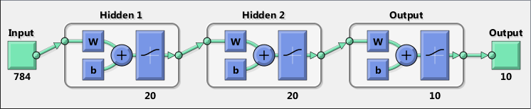
When done you can use the view function, and you should now have something similar to this:

% View the network
view(net2)

As you have probably noticed, the number of inputs and outputs is not configured yet, as indicated by the zeros associated with the input and output. However, this can be automatically configured by the training dataset, as the number of rows in the transformed images data input is 784, and the number of rows in the transformed label data is 10.

The Matlab function for this is called configure:

% Use the configure function to set the number of inputs and outputs
% according to the training data
net3=configure(net2,training_images,training_labels);
view(net3);

Here 'training_images' is the transformed training images (784x60000) and 'training_labels' is the transformed training labels (10x60000), both of which you should have created in Part 2

Part 5 - Setting the initial weights and biases

Your network is now almost ready to be trained. However, the last thing you need to do before training is to specify initial values of the weights and biases in the network. By default, all weights and biases are set to zero, which is a very bad starting point for the numerical minimisation algorithm, because if a large fraction of the weights and biases are zero, it is very likely that the cost-function is insensitive to changes of the parameters. The actual initial values of the weights and biases are not important, as long not all of them are zero. It is also a good idea to have both positive and negative initial values.

Therefore you want to set all initial values for the network weights and biases to a random number between -1 and 1. In Matlab, such a random number can be generated using the rand function. The rand function gives a uniform distributed random number in the interval (0,1), which can be transformed to the interval (-1,1) instead.

% This will output 10 uniform random numbers between -1 and 1 in one column
% vector
-1+(2)*rand(10,1)

ans =

    0.4368
    0.0631
    0.5397
    0.9007
   -0.0486
   -0.5532
    0.5636
   -0.4477
   -0.9260
    0.2200

The weights applied to the input, when it goes into the first hidden layer are found in net.IW. The weights applied in the process between layers are found in net.LW. Lastly, all the biases are found in net.b.

% Here are the weights of the input into the first hidden layer:
net3.IW
% Here are the weights applied between layers:
net3.LW
% Here are alle the biases of the network;
net3.b

ans =

  3×1 cell array

    {20×784 double}
    { 0×0   double}
    { 0×0   double}


ans =

  3×3 cell array

    { 0×0  double}    { 0×0  double}    {0×0 double}
    {20×20 double}    { 0×0  double}    {0×0 double}
    { 0×0  double}    {10×20 double}    {0×0 double}


ans =

  3×1 cell array

    {20×1 double}
    {20×1 double}
    {10×1 double}

As you can see the input weights, layer weights and the network biases are arranged in a Cell-structures, of which some cells are empty { 0x0 double}. This is because Matlab can work with Neural Networks that are much more complicated and less straightforward, than the one you are using in this exercise. However, it is important, that you only insert random numbers between -1 and 1 in non-empty cells and without changing the dimension of the matrix inside the cells.

% This is an example of how you can set the initial input weights
% without changing its dimension
net3.IW{1}=-1+(2)*rand(size(net3.IW{1}));

You can use similar approach to set initial weights and biases values in:

net3.LW{2}
net3.b{1}
net3.b{2}

When you are done your are ready to train your Network!

Part 6 - Network Training

The function for training Neural Networks in Matlab is called train. A long with the network you want to train, you need to input the transformed training images and transformed labels.

% This will start the network training and open the network training tool
net=train(net,training_images,training_labels);
% You do not need this line - I just need it to show network training tool
% as an image in this exercise :)
nntraintool;

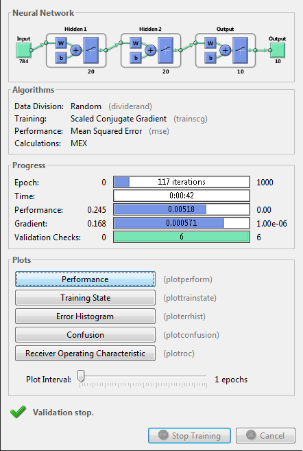
Spend some time to review the different performance plots while the network is training. You specified these five performance plots in Part 4

Part 7 - Using the trained network on new data and tests its performance

In this part we want to test the performance of your Neural Network, and for this purpose, you need to load the 10.000 test images and labels found in:

You can use the same loading function, as you used in Part 1 to load the training data.

When you have your trained network, it is very easy to classify and recognise new images. The network can be called as a standard function in Matlab:

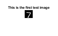
% Here the trained network is used to recognise the first images of
% the test data
imshow(test_images(:,:,1)); title('This is the first test image');
% The first image is transformed to a colum vector
Col_img=reshape(test_images(:,:,1),[],1);

% The neural network is used to recognise the digit
y=net(Col_img);
% This is the answer from the neural network
disp(y);

    0.0103
    0.0000
    0.0000
    0.0001
    0.0000
    0.0000
    0.0000
    0.9966
    0.0000
    0.0012

Because the network gives the highest value in row number 8, the Neural Network classifies the digit on the image correctly as a number 7.

Now you need to use your trained classification neural network to classify all the 10.000 test images and compare the result with their labelled value to calculate the performance. Meaning, how many % is recognised correctly of the 10.000 test images? Remember the 10.000 test images have not been used in the training process, so a test like this is objectively expressing the performance of your network.

Try also to plot the images of 5 to 6 digits the Neural Network misclassify, so you can judge whether or not it is fair, that the network fails.

Part 8 - Matlab Neural Network toolbox

Matlab has some Neural Network Apps (toolboxes), that can turn out to be very handy for you, if you want to apply Machine Learning and Neural Network in your project.

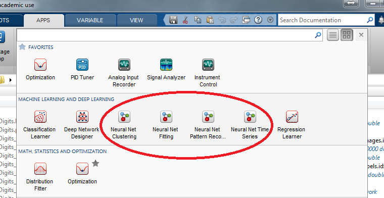
Dependent on the kind of data problem you are working with, Matlab has some standard networks optimised for different applications.

These are all implemented as APPs with a graphical user interface (GUI) that can help you build, test and design the Neural Network to your application. The problem you have worked with in this exercise is pattern recognition.

Therefore, try to use the Neural Network App for Pattern Recognition to create a network that can classify the handwritten digits. Compare the network with your regarding:

% Ths commands opens the Neural Network Pattern Reconition APP
nprtool;

%test

Published with MATLAB® R2018b